We make it easy for students, faculty, and researchers to work with mathematical optimization. The example will install the gurobipy package, which includes a limited Gurobi license that allows you to solve small models. We look forward to sharing our expertise, consulting you about your product idea, or helping you find the right solution for an existing project. And we get the lowest cost of transportation of 16 thousand dollars. Or-tools Google’s software suite for combinatorial optimization. This is an open-source, fast, and portable software suite for solving combinatorial optimization problems.

#Both labor and material are required for producing the products ‚S’ and ‚T’. We then explore the code examples, with elaborative examples to understand the various scenario where the liner programming can be utilized. Thus, it is reasonable that the loan amounts at the beginning of the first and second year are valueless.

Complete linear programming solver code in Python

Because $x_$ has a negative coefficient in the objective, the optimization will minimize $x_$. The presolve time was only 1.32 seconds and reduced the solution time from nearly half an hour to under 25 seconds. Most of the CPLEX Optimizers for MP call upon the basic simplex method or some variation of it.

Linear programming is where we find optimal values in a feasible vector space defined by constraints represented as linear equations. The most intuitive form of constraints may be nonlinear, but can be derived into a linear form for the purpose of the linear program. During my time working in fundraising, I worked on the web development side, building and maintaining websites and tools for public and internal use. Many of the problems that kept coming up in my department were optimization problems, many of which were directly related to business operations.

This problem is to maximize the objective, so that we need to put a minus sign in front of parameter vector c. The optimal plan tells the factory to produce 2.5 units of Product 1 and 5 units of Product 2; that generates a maximizing value of revenue of 27.5. The blue region is the feasible set within which all constraints are satisfied. Other solvers are available such as SCIP, an excellent non-commercial solver created in 2005 and updated and maintained to this day.

More from Towards Data Science

Then you’ll explore how to implement linear programming techniques in Python. Finally, you’ll look at resources and libraries to help further your linear programming journey. The Python ecosystem offers several comprehensive and powerful tools for linear programming. You can choose between simple and complex tools as well as between free and commercial ones. The highlighted area shows the set of decisions about $s$ and $t$ which satisfy all of the constraints — this is the feasible region. Formulate a mathematical model of Giapetto’s situation that can be used to maximize Giapetto’s weekly profit.

Prob.objective holds the value of the objective function, prob.constraints contains the values of the slack variables (we don’t require them but just a good to know fact). Mixed-integer linear programming allows for overcoming many demerits of linear programming. One can approximate non-linear functions withpiecewise linear functions, model-logical constraints (ayes/no problem like whether a customer will churn or not), and more. Our specialists from Svitla Systems are very well versed in solving such problems. This allows us to quickly and efficiently solve the problems encountered by our customers. This example was considered for demonstration, but in fact, this approach allows us to solve problems with millions of components, for example, in a transport problem.

Because the cost should be minimal, at the same time, deriving the nutritional value from the combination of different food items should be maximum, considering the maximum and minimum constraints given in the data. A nutritional component’s minimum and maximum bounds define the inequality constraints. The optimization problem seeks a solution to either minimize or maximize the objective function, while satisfying all the constraints. Such a desirable solution is called optimum or optimal solution — the best possible from all candidate solutions measured by the value of the objective function. The variables in the model are typically defined to be non-negative real numbers.

The variables used in the linear-optimization model of the production problem are called primal variables and their solution values directly solve the optimization problem. The linear-optimization model in this setting is called the primal model. Pyomo is a good choice for modelling complex optimization problems. It interfaces a wide range of optimization solvers, not just limited to linear solvers. For simple LP problems, we can declare expressions explicitly like the example below. We can also generate rule-based expressions for the objective function and constraints using Python functions .

Hands-On Linear Programming: Optimization With Python

Numpy is an array library, with some extra functionality tossed in for backwards compatibility. Scipy has some optimization routines, but as of now I think it’s only general non-linear solvers. Scipy does not currently have a solver specialized for linear programs. Looks like there’s a pull request to scipy containing a linear programming implementation, though. So a linear programming solver could be in scipy in the future. You want to minimize the cost of shipping goods from 2 different warehouses to 4 different customers.

In summary, the maximum profit a company can make is $155.45 while producing 31.82 cups and 30 plates. Demand for cups is unlimited, but demand for plates is 30 units. It is widely used to solve optimization problems in many industries.

First and extra linear optimization python for overtime, with an upper bound of 100. $$ overtime Finally, add an additional cost to the objective to penalize use of overtime. DOcplex helps you identify potential causes of infeasibilities, and it will also suggest changes to make the model feasible. A constraint is binding if the constraint becomes an equality when the solution values are substituted. If you’re using a Community Edition of CPLEX runtimes, depending on the size of the problem, the solve stage may fail and will need a paying subscription or product installation.

Nutrient data example

Minimization concerning linear programming in Python means to minimize the total cost of production whereas Maximization on the other hand means to maximize the company or organization’s profit. Hence, linear programming in Python with its graphical method helps to find the optimum solution. Now we create a list of all the food items and thereafter create dictionaries of these food items with all the remaining columns. The columns denote the nutrition components or the decision variables here.

• The feasible solution that corresponds to maximal z is the optimal solution.
• You can get the optimization results as the attributes of the model.
• It will connect to the COIN-OR Linear Programming Solver for linear relaxations.
• The continuous variable cell represents the production of cell phones.

As you can see, the simplex method traverses the edge of the feasible region, while the barrier method moves through the interior, with a predictor-corrector determining the path. In general, it’s a good idea to experiment with different algorithms in CPLEX when trying to improve performance. It is possible that multiple non-optimal solutions with the same objective value exist. The simplex algorithm works by finding a feasible solution and moving progressively toward optimality. Where $x$ denotes the vector of variables with size $n$, $A$ denotes the matrix of constraint coefficients, with $m$ rows and $n$ columns and $B$ is a vector of numbers with size $m$.

A quick guide for Linear Programming using Python (PuLP). – mnips/Linear-Programming-Python-1

Graph representation for a multicommodity transportation problem. Suppliers are represented as squares and clients as circles; thick lines represent arcs actually used for transportation in a possible solution, and colors in arcs mean different products. This represents the amount of reduction on costs when increasing the capacity constraint by one unit . The first lines, not shown, report progress of the SCIP solver while lines 2 to 6 correspond to the output instructions of lines 14 to 16 of the previous program.

And raw materials from a warehouse of 2 and warehouse 1 of 4 tons are brought to the second plant. That is, each plant will receive 8 tons of raw materials, as was necessary. There is some uniform cargo that needs to be transported from n warehouses to m plants. For each warehouse i it is known how much cargo ai is in it, and for each plant its need bj for cargo is known. The transportation cost is proportional to the distance from the warehouse to the plant (all distances cij from the i-th warehouse to the j-th plant are known).

• By default, PuLP uses the CBC solver, but we can initiate other solvers as well like GLPK, Gurobi etc.
• Therefore, in general, solving integer-optimization models is much harder.
• We provide a standard form of a linear program and methods to transform other forms of linear programming problems into a standard form.
• The optimal solution corresponds to the point in the feasible region that maximizes the value of y.
• In the earlier example you saw how one can visualize multiple optimal solutions for an LP with two variables.

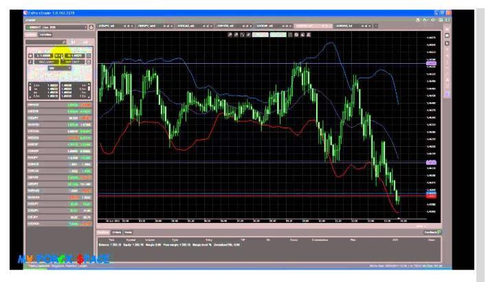
The https://forexhero.info/ of a variable gives an indication of the amount the objective will change with a unit increase in the variable value. It then moves from one vertex to another, gradually decreasing the infeasibility while maintaining optimality, until an optimal feasible solution to the primal problem is found. In any solution to the dual, the values of the dual variables are known as the dual prices, also called shadow prices. To improve the efficiency of the simplex algorithm, George Dantzig and W. CPLEX uses the revised simplex algorithm, with a number of improvements. The CPLEX Optimizers are particularly efficient and can solve very large problems rapidly.